The EXTraS project. Exploring the X-ray transient and variable sky - Notes on De Luca et al. 2021

The Idea

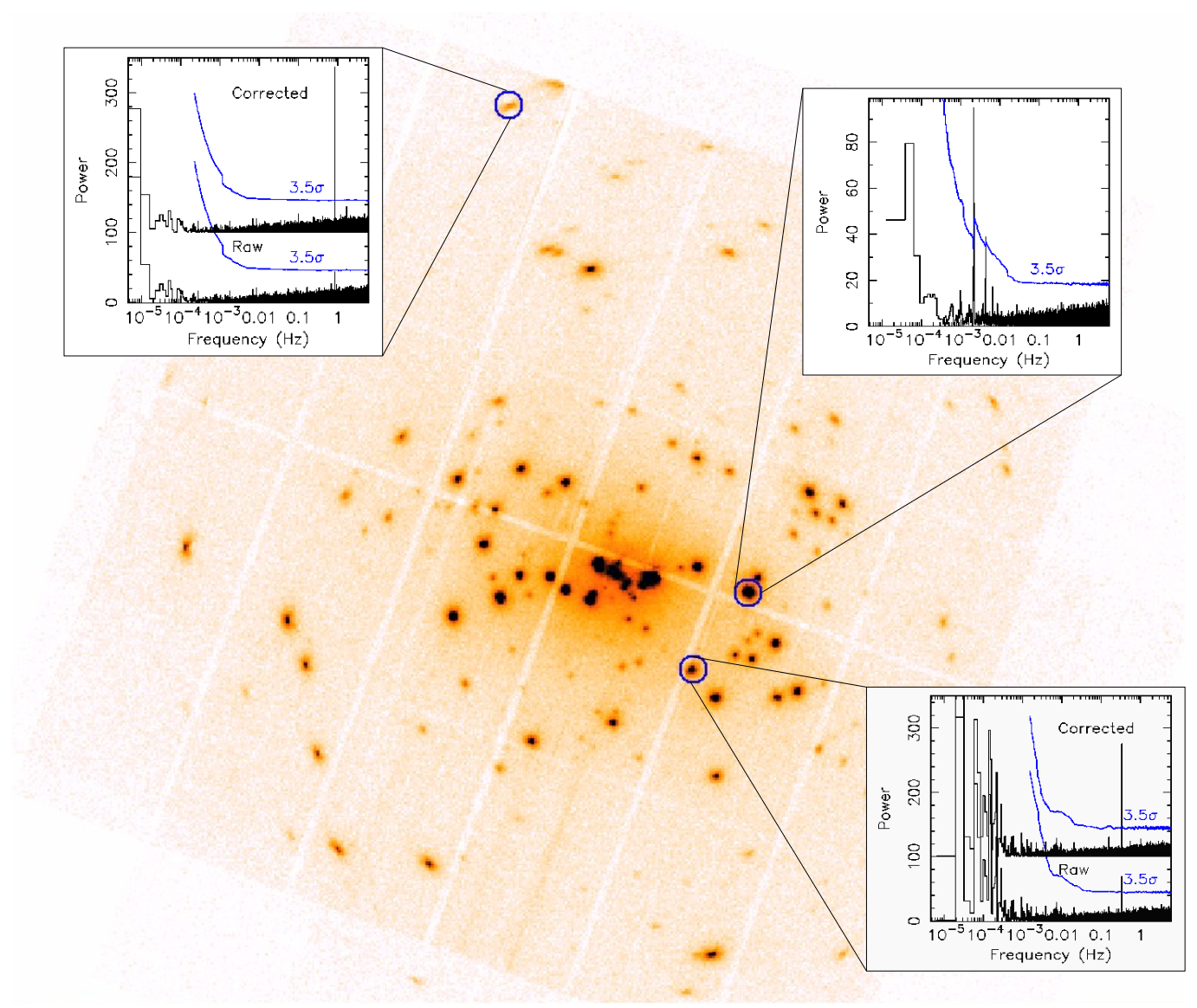
From 2014 to 2016, “The EXTraS project: Exploring the X-ray transient and variable sky” was carried out and produced a variety of results. This paper gives an overview of the project, summarizes these results and gives some pointers on where to find products, results and more.

Context

The sky, especially the X-ray sky, is highly variable on a wide range of timescales, and by studying the variability we can learn more about the nature and emission physics of the sources responsible. Some of these sources are

1. Gamma-ray bursts (GRBs), which are likely to be produced by the collapse of massive stars into black holes, or by the merger of two neutron stars.
2. Soft Gamma Ray Repeaters (SGRs), which are powered by magnetars.
3. (Transient) X-ray binaries with black holes, neutron stars or white dwarfs accreting matter from their stellar companion.
4. Stellar flares (in X-rays) from magnetically active stars (either isolated or in binary systems).
5. Blazar flares, which I had never heard of before, but that is because they are gamma-ray flares produced by jets from supermassive black holes at the centres of galaxies (and therefore much larger objects than I have dealt with so far).
6. Tidal disruption events, which occur when a star is tidally disrupted by a supermassive black hole.
7. Supernova X-ray flashes, produced by the supernova shock emerging from the exploding star.

Some possible causes for the time variability of number 3 are then listed, if I understand correctly, although I’m not sure why these are singled out. But the fact is that the rotation of a star or a compact object, as well as its orbital motion in a binary system, can give rise to a variety of time variability properties. And we need to understand this time variability if we are to understand the nature and physics of these sources.

Large field-of-view instruments are ideal for such studies, but focusing telescopes such as XMM-Newton have been around long enough to accumulate large archives of many serendipitous X-ray sources that can also be studied. EXTraS aims to take advantage of this. In most cases, the time binning is 1.46 seconds, or a time bin is long enough that there are on average at least 20 counts per bin. This is a limiting factor of the instrument and science can only be done on longer time scales.

A little more detail: What did EXTraS do?

EXTraS looked at the database of the EPIC instrument on XMM-Newton and looked at four different areas of the problem:

1. Short-term, aperiodic variability (STV): find as many sources as possible, on all timescales (from the instrument’s time resolution to the duration of an observation).
2. Search for coherent pulsations: find as many X-ray pulsators as possible, with a period range from 0.2 seconds upwards (although I’m not sure how this fits with the time binning of 1.46 seconds mentioned above), up to the highest possible value during an observation.
3. Search for transients: find as many new X-ray transients as possible.
4. Long-term variability (LTV): find variability in overlapping observations, at different epochs (up to 15 years).

All the results of these sub-projects have been published online, together with a database of temporal properties and supplementary files. This paper explores these different areas in more detail, including the results and examples of the science that can be done with the results. I will only discuss the “search for new transients” (section 5 of the paper).

Searching for new transients

New X-ray transients can only be found by examining short time intervals, but not by time-integrated analysis of the entire XMM observation. To identify good time intervals, they used a Bayesian block analysis of the time variability in different regions of the EPIC detector. The steps of the analysis are

1. Data cleaning and preparation.
2. Time interval construction and source detection.
3. Position matching to identify transient sources.
4. Position matching to compare results in different instruments, bands and catalogues.

The software they use for their pipeline is a mixture of C shell scripts, C++, Python, FTOOLS and SAS.

As a result, EXTraS produced a catalogue of 136 transient sources, which they made available as a FITS file in the database, along with some BITMAP and ASCII files for each source. Unfortunately, however, the EXTraS web site and Public Data Archive has been offline since June 2022 (lack of funding to maintain such a thing?).

Follow-up

• Machine learning algorithms have also been used to characterize sources based on catalogues and phenomenological classification. This is not presented in this paper, but the authors refer to Gatuzz et al. (2018) for more information.
• What are Bayesian block light curves? Quote from the paper: “Bayesian block is a well-known adaptive-binning algorithm that finds the statistically significant count rate change-points by maximising the fitness function for a piecewise-constant representation of the data, starting from an event list.”
• In their Figure 9 they point out that flares, for example, are missed because in the XMM catalogue they only calculate the variability with respect to the good time intervals. But the good time intervals are there for a good reason, I haven’t figured out how they deal with that and how they can come to their conclusions (I assume they don’t just ignore the good time intervals).

Keep in mind

• They discuss an issue for the pn camera, where a known bug in the product generation pipeline can cause incorrect time tagging of an event within an exposure, and therefore the timing analysis cannot be performed.
• They have also implemented a different approach to background modeling, which I might keep in mind for future analysis.
• Maybe I should learn some basic C++.